Building Three Tangled Agents
A software agent is an artificial intelligence software program designed to take actions (ie have agency) in response to the state of their environment.
Let’s look at how to build game-playing agents for any Tangled game board. We can then play against these agents, and agents can play against each other!
Building game-playing agents
The API for a Tangled agent is really simple. Given the current game state, which is a list of N+E integers, select and return an integer in the range 0..N+3E-1 representing an action allowed from that game state. The actions numbered from 0 to N-1 correspond to choosing the corresponding vertex, and the actions numbered from N to N+3E-1 correspond to selecting integers 1, 2, or 3 for the edges in dictionary order.
For example, if V=3 and E=3, game state is [V₀, V₁, V₂, e₀₁, e₀₂, e₁₂], and action 0 selects V₀ to be the player number (either 1 or 2 for a two-player game); action 1 selects V₁; action 2 selects V₂; action 3 chooses e₀₁ to be 1; action 4 chooses e₀₁ to be 2; action 5 chooses e₀₁ to be 3; action 6 chooses e₀₂ to be 1; action 7 chooses e₀₂ to be 2; action 8 chooses e₀₂ to be 3; action 9 chooses e₁₂ to be 1; action 10 chooses e₁₂ to be 2; and finally action 11 chooses e₁₂ to be 3.
So an agent is a map from a list of N+E integers to a single integer in the range 0..N+3E-1. That’s it!
Here’s an example full game sequence, where the move made at every step is singled out in purple above the corresponding game graph.

Left: a sequence of moves, shown as (top) state changes where the most recent change is shown in purple and (bottom) the game board for those states. Right: the states, ordered from beginning (top) to end (bottom), as a matrix. The actions selected here are, in order, 4, 9, 0, 2, and 6; so the red agent returned action 4 from state [0,0,0,0,0,0]; action 0 from state [0,0,0,2,0,1] and action 6 from state [1,0,2,2,0,1]. The blue agent returned action 9 from state [0,0,0,2,0,0] and action 2 from state [1,0,0,2,0,1].
To decide how to move, an agent only needs to know the current state and some information about the game board — the game is Markovian (the path to the current state doesn’t matter). As shown above on the right, each game can be recorded as a matrix where the rows are the state of the game at each turn, and there are P+E rows (if we ignore the first row which is always all zeros), where E is the number of edges in the graph and P is the number of players, (2+3=5 in this case).
A Random Agent
The easiest agent to build selects random moves from the set of allowed moves at every turn. Here is my random agent:
def agent_random(state):

    possible_moves = all_allowed_moves_from_this_state(state)

    if len(possible_moves) > 0:
        return random.choice(possible_moves)
    else:
        return None   # game over -- no valid moves -- this was a terminal state
The all_allowed_moves_from_this_state(state) function returns all the allowed subsequent moves from the current state of the game, which is easy to implement. If there are no allowed moves then the game is over, and the agent returns None, and we know state is a terminal state.
A Monte Carlo Tree Search Agent
The random agent will be useful for a baseline but not much else. Let’s build a Monte Carlo Tree Search (MCTS) based agent that can potentially play well.
If you are new to MCTS, I’d recommend reading the Wikipedia article linked above — it’s pretty good. I won’t go into it here in much detail, as there are many great tutorials and explanations available, and I won’t be able to do better. But one thing I would like to highlight is that evaluation of terminal states is a very important part of this algorithm. Here’s a summary of how the algorithm works in picture format:

The MCTS algorithm has four phases that repeat until you run out of time and/or patience. The key step to highlight here is the third one (rollout). In this phase, some policy (e.g. random choice) is applied to both players, starting from some initial state (the dark circle) and ending at that game’s terminal state. The terminal state is evaluated (win/lose/draw) and then in phase four the result is backpropagated up the chain to make it more likely that actions resulting in wins for the AI currently taking an action are more likely to be taken, and actions resulting in losses are less likely to be selected. If evaluating the terminal state is hard, MCTS gets bottlenecked by this third phase.
In order to make a good guess at what move to take from any given state (in the case of the image above, we want to know what action/move to take from state s₀), we need to do many iterations of the four phases above in order to get a good sampling of the possible results of taking all the possible actions from that state. A way to parametrize MCTS is to select how many iterations of the above four phases we will allow before selecting an action — more is better. If we call this number R, then we need to evaluate R terminal states for each move selected. If evaluating a terminal state is costly (and that’s what we’re trying to achieve with Tangled), then doing it R times is even harder!
We can store the result of each terminal state evaluation if we want to, but this only makes sense for small graphs (the three- and four-vertex ones we’ve looked at are fine, but anything bigger becomes intractable). The number of possible terminal states quickly becomes staggeringly large in Tangled and you’ll likely never see the same one twice.
In my MCTS implementation, I use the Upper Confidence Bound (UCB) algorithm to explore/exploit different action choices from each state. There are lots of good write-ups of how UCB works. Usually, UCB is introduced using the multi-armed bandits problem. This is the same problem we face when deciding what action to take — given several slot machines, each with different payoffs which we don’t know, which do we try in which order to find the machine with the best payoff. That’s what UCB tries to do!
An Optimal Policy Agent, and MCTS’ connection to Q-Learning
In MCTS (and games/life in general!) we want to know what action a to take from state s₀ to maximize some measure of goodness. In games, this measure is connected to winning, losing, or tying a game.
A function called the quality of a state/action pair, denoted Q(s₀, a), is approximated by the MCTS algorithm by running P simulated games unrolled from the initial state s₀. In the limit where P → ∞, the probabilities of winning by taking any action a computed using MCTS approximate the optimal quality Q*(s₀, a) giving the optimal policy 𝛑*(s₀) = max ₐ Q*(s₀, a) (ie the policy at any state is to select action a for which Q*(s₀, a) is largest).
The quality Q is what is learned using Q-learning, a basic but powerful family of reinforcement learning algorithms. Q-learning is much more useful when we don’t have a model of the environment and / or the effect of actions are stochastic — neither of these is true for Tangled! So you could use Q-learning algorithms here to find Q*, but since we have a model of the environment and actions are deterministic it’s more efficient to use MCTS planning/search to approximate Q* than use model-free learning.
In MCTS, Q(s₀, a) is usually thrown away once we’ve taken the action. We can instead store the Q(s₀, a) values for each state s₀ we visit. If we do this we are building a Q-table, which is valuable for at least two purposes.
Reason 1: If the game graph is small, we can enumerate all the states a player could see and calculate Q(s₀, a) for all possible state/action pairs. This will result in the limit of large enough P (from the experiments below, it looks like P ~ 500 is good enough for these two graphs) in an optimal policy (from any state s, select the action a that maximizes Q(s, a)). The advantage of this approach is that once we’ve built the full Q-table, the optimal policy can be executed using a simple look-up instead of having to constantly re-calculate every time.
This strategy only works for tiny graphs. Once the graphs get bigger, tabular methods fail as the state space grows exponentially (~ 3ᴱ) with edge count.
Reason 2: The quality values generated by MCTS can be used in a more sophisticated way by combining MCTS with neural nets. This is the premise of AlphaZero and its cousins. We will revisit this as we build more sophisticated game-playing agents shortly!
Comparing These Agents on Tiny Graphs
At least for small graphs, we can enumerate who wins from all the terminal states, store these, and then use them as lookup tables. When we can pre-compute who won from each terminal state, it’s easy to run AI vs AI competitions as the evaluation of terminal states is just a lookup.
Unfortunately, the number of graphs where we can build a full lookup table is limited. The number of terminal states and the cost of evaluating each both grow exponentially, with edge count and vertex count respectively. We can easily run competitions on both of the graphs we’ve already looked at. Anything bigger is prohibitive for the setup we’ve been considering so far, adn we’ll have to get smart about terminal state evaluation.
The two graphs we will examine gameplay on here are the three-vertex three-edge and the four-vertex six-edge graphs.
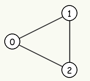
The three-vertex, three-edge graph
The first graph we’ll look at is the three-vertex one, where we’ll set up competitions between random and MCTS agents to see how they do against each other.
MCTS is parametrized by either the number of rollouts (equivalently, how many times through the four phases of the algorithm we allow) or a timeout in seconds. Increasing either increases the performance of the algorithm. These costs are incurred during runtime.
Random vs Random
The first thing I wanted to check was that all the machinery for coding up the headless AI vs AI agents was working. I ran one million random (red) vs random (blue) games and got 259,088 red wins, 258,668 blue wins, and 482,244 draws. If we compare these results to the distribution of terminal states we computed in one of my earlier posts we had 25.9% red wins, 25.9% blue wins, and 48.1% draws, so the random vs random numbers look correct. Yey!
Random vs MCTS
Now we’ll run MCTS against the random agent. We parametrize MCTS by the number of rollouts. We also need to specify which player is which, as who goes first may be important. I ran 1,000 trials for each competitive pairing. Here are the results.

Results of random vs MCTS agents on the three-vertex three-edge graph.
One puzzling thing is that one rollout MCTS does worse than random both going first and second, and when pitted against each other always give draws. There’s something pathological about my MCTS implementation when there’s only one rollout — something to check! Other than that, everything looks believable. We can see that being red and going first (and also having 3 moves vs blue’s 2) provides an advantage on this graph, but in the limit of good play (high rollout MCTS vs itself), even disadvantaged, blue can always force a draw. 100 rollout red never loses to random blue, and 1,000 rollout blue never loses to random red. 1,000 rollouts seem to be enough to play optimally for both sides.
Random & MCTS vs Pre-Computed Optimal Policy 𝛑*
For each possible game state s₀, I ran MCTS for 10,000 rollouts and stored the resultant entries in the Q-table for each action from that state. This pre-computes Q*(s₀, a) and therefore the optimal policy 𝛑*(s₀) = maxₐ Q*(s₀, a).
I ran 1,000,000 games playing the optimal policy against the random agent. For random red vs optimal blue, I got 687,440 blue wins and 312,560 draws. For random blue and optimal red, I got 759,512 red wins and 240,488 draws. So far so good — we don’t want a random agent beating our supposedly optimal policy!
Next, I ran the (presumably, allegedly) optimal policy against MCTS agents with different numbers of rollouts, playing vs. MCTS as both red and blue.
Against MCTS with different numbers of rollouts, I got these results:

As a check, I also ran vs. 20,000 rollout MCTS (twice what I used to get the optimal policy) and got 1,000 draws for MCTS playing both red and blue, so it’s likely generating Q* using 10,000 rollouts per state is sufficient to get an optimal policy for this game graph. It looks from these results like this could be optimal for both red and blue — I didn’t see a single loss in any experiment I tried for the optimal policy playing as either red or blue.
Observations for Tangled on The Three Vertex Graph
Here are some takeaways from these experiments:
Playing as red provides a significant advantage — two possible reasons: (1) going first and (2) since there are only 5 moves per game, you get 3 moves including first and last whereas blue only gets 2 moves.
The optimal policy does seem optimal — it never lost once even when playing as disadvantaged blue, even against a 20,000 rollout MCTS opponent playing red.
The four-vertex, six-edge graph
The second graph we’ll look at is the four-vertex one.

We can perform the same analysis we did one the last graph. Here are the results!
Random vs Random
I ran one million random (red) vs random (blue) games and got 186,742 red wins, 188,688 blue wins, and 624,570 draws. If we compare to the distribution of terminal states we computed in one of my earlier posts we had 18.8% red wins, 18.8% blue wins, and 62.4% draws. All good!
Random vs MCTS
Same as for the smaller graph, here are the results of running MCTS against the random agent. We can see here that the 1 rollout results look weird here also. For everything else we can see that blue has an advantage. Note that here there are 8 total moves, meaning blue goes last. For the previous graph there were 5 total moves, red went last, and red had an advantage. When both players are playing well, red can always force a draw. Somewhere between 100 and 1,000 rollouts likely guarantees worst case a draw for the AI, regardless of whether red or blue is played.

Results of random vs MCTS agents on the four vertex six edge graph.
Random & MCTS vs Pre-Computed Optimal Policy 𝛑*
I did the same thing here as I did for graph 2 — for each possible game state s₀, I ran MCTS for 10,000 rollouts and stored the resultant entries in the Q-table for each action from that state. Like for graph 2, this presumably pre-computes Q*(s₀, a) and therefore the optimal policy 𝛑*(s₀) = maxₐ Q*(s₀, a).
I ran 1,000,000 games playing the optimal policy against the random agent. For random red vs optimal blue, I got 697,665 blue wins and 302,335 draws. For random blue and optimal red, I got 607,022 red wins and 392,978 draws.
Next, I ran the optimal policy against MCTS agents with different numbers of rollouts, playing vs. MCTS as both red and blue.
Against MCTS with different numbers of rollouts, I got these results:

I also ran vs. 20,000 rollout MCTS (twice what I used to get the optimal policy) and got 1,000 draws for MCTS playing both red and blue, so it’s likely generating Q* using 10,000 rollouts per state is sufficient to get an optimal policy for this game graph also. It looks from these results like this could be optimal for both red and blue — I didn’t see a single loss in any experiment I tried for the optimal policy playing as either red or blue.
Observations for Tangled on The Four Vertex Graph
Here are some takeaways from these experiments:
Unlike graph 2, playing as blue provides a significant advantage this time. As both players get 4 moves each, the only obvious difference is that blue goes last — this could be the source of the advantage. This is a commonality of the graph 2 situation where red went last and had an advantage.
The optimal policy does seem optimal — it never lost once even when playing as disadvantaged red, even against a 20,000 rollout MCTS opponent playing blue.
Summary
We now have three agents to play Tangled with, a random agent, an online MCTS agent, and a pre-computed optimal agent. The first two strategies should work for larger game graphs, but pre-computing all possible Q values only works for tiny graphs — it’s unlikely we will be able to discover optimal policies for anything ‘reasonable sized’.
For both N=3 and N=4 complete graphs, the player going last has a significant advantage. It’s unclear whether this is just a quirk of the small graph size or whether this might persist to larger game graphs.