Adjudicating Tangled Terminal States on Tiny Graphs With Three Different Approaches

Tangled is based on the assumption that quantum supremacy can be achieved by sampling the output distributions of a D-Wave quantum computer after a quantum quench. This claim depends on us not being able to effectively spoof this output using some other approach.

I’ve been using three different approaches so far to adjudicate Tangled terminal states. Here I’ll describe what they are, and compare their results on the teeny tiny three- and four-vertex graphs.

I’m also providing code that implements all three solvers, so you can try all of this yourself!

Approach #1

The first approach is a numerical Schrodinger Equation solver. This only works for tiny game graphs as the compute time grows exponentially with vertex count, so will not be an option as the graphs get bigger. I won’t describe this one too much as it’s pretty basic and it’s not relevant to anything of the size we are ultimately after. I’ll include results from its use for the tiny graphs just to double check agreement but post that we won’t be able to use it!

Approach #2

My main debugging workhorse right now is a specially tuned simulated thermal annealing (SA) variant run on the classical s=1 limit of the Hamiltonian

SA is a heuristic algorithm for first generating an approximation to a low-temperature Boltzmann distribution (over the states whose energies are given by the above expression) and then drawing samples from it. The Boltzmann distribution here could be ‘similar enough’ to the probability distribution after the quantum quench to get most/all the terminal state adjudications right.

The variant I’m using is based on the D-Wave simulated annealing code with a specific choice of annealing schedule that they came up with that is supposed to reproduce the hardware distribution as closely as possible. I’ve been using it pretty extensively.

Investigating the performance of this approach carefully is important as the D-Wave quantum supremacy claim requires this (and any other classical approach!) to fail for large graphs. I think it will, but if it does, we need to measure this and explain why it’s failing.

Approach #3

The ground truth for Tangled terminal state adjudication is the mighty D-Wave Advantage2.5 system, using Algorithm 1 described in this post.

We’ve got three different approaches locked and loaded to evaluate Tangled terminal states. Let’s see how they do!

Evaluating Tangled Scores for All 27 Unique Terminal States for The Three Vertex Graph

I adjudicated all 27 unique terminal states of the three-vertex graph using the three different approaches I listed above. For the SA algorithm, I drew a huge number (N=10,000,000) of samples per problem (why not, it’s cheap). The width of the distribution around each answer is proportional to the square root of N, so with a huge N like this we’re pretty sure we are getting something close to the true mean of the distributions around each problem.

For the D-Wave Advantage2.5 quantum computer, I embedded each 3-variable problem in P=343 parallel places on each chip, used M=1 automorphisms, turned off gauge transforms and shimming, and gathered N=1,000 samples from each run, giving a total of MxNxP=343,000 samples per problem. This is quite a bit fewer than the SA run, but that was overkill anyway!

Here’s the results for the scores for all 27 problems. I’m displaying this as a stacked histogram using 200 bins to cover the entire range of possible scores -2<R<+2. You can see good agreement for the computed scores for all states for all three methods. The green dashed lines are the borders that distinguish draws from wins, and you can see none of the methods return scores that are close to these borders, so all three agree on the adjudications of all of the states.

I ran all three solver methods to adjudicate all 27 unique terminal states for the three-vertex graph. This is a stacked histogram with the results using 200 bins. Also included are green dotted lines denoting the border between wins and draws (anything in between the green lines is a draw). You can see that all solvers agree on win/loss/draw for all terminal states.

What Terminal States Are Near ±2/3?

I looked at which states were the ones scoring ±2/3 — these are the states nearest the draw line. The two unique states giving scores of + 2/3 and -2/3 respectively are [0, 1, 2, 2, 3, 2] and [0, 1, 2, 3, 2, 2].

I worked out the energies, correlations and influence scores for the top graph (state [0, 1, 2, 2, 3, 2]) (bottom one is similar but correlation between 0 and 1 is negative, correlation between 0 and 2 and 1 and 2 are positive, and influence is zero except for site 2 where it's positive).

Evaluating Tangled Scores for All 729 Terminal States for The Four Vertex Graph

I adjudicated all 729 unique terminal states of the four-vertex graph using the same three approaches. Again I got good agreement, with zero disagreements between adjudicators.

For the D-Wave Advantage2.5 quantum computer, I embedded each 4-variable problem in P=215 parallel places on each chip, used M=1 automorphisms, turned off gauge transforms and shimming, and gathered N=1,000 samples from each run, giving a total of MxNxP=215,000 samples per problem.

Here’s what I got:

Some interesting stuff here! Like what’s up with the big simulated annealing spikes near ±4/3 without accompanying quantum samples? And also why are the cyan samples not stacked on the ±2/3 result? What’s with the clumps of cyan around ±5/2?

A Very Interesting Type of State

That big spike of red around ±4/3 needs a closer look. There are a few of them but let’s just narrow in on one of them for now.

This is one of the states in the red spike at score ~ -4/3. The instance has six ground states, resulting in the simulated annealer equally sampling from all six, producing an influence vector of (1,1,-1/3,1) and a score of -4/3. But this is not what the Schrodinger solver returns. Instead, in the adiabatic (long anneal time) limit, the highlighted states (1,1,-1,1) and (-1,-1,1,-1) are twice as likely as the other four, giving a different influence vector of (1,1,-1,1), and a score of -2!

This is an example of a Tangled game state whose score obtained from using simulated annealing and the score obtained from coherent quantum evolution are different. The mechanism for the difference is an interesting quantum mechanical effect related to the number of bit flips between the ground states.

To see what’s going on, let me construct an adjacency matrix over all six ground states, where the entries of the matrix are 1 if the states are only one spin flip apart, and 0 otherwise. The matrix in this case looks like this:

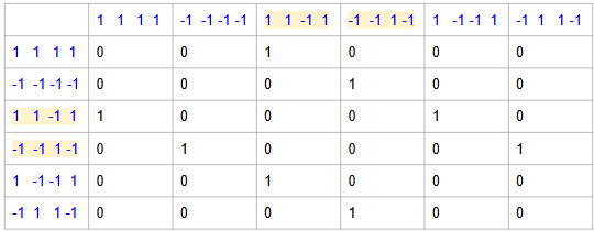
Note that the highlighted states are 1 spin flip away from two different states, whereas the non-highlighted ones are 1 spin flip away from only one. The transverse term in the Hamiltonian splits these six states, putting more weight into states that have more 1-spin-flip connections to other states in the groundstate bundle. This is a quantum mechanical effect, and predicts the probabilities to be 1/8 for the unfavored states and 1/4 for the favored ones in the adiabatic limit, which is what I observe with the Schrodinger solver.

This is super cool as it’s a small instance where simulated annealing fails for an obvious reason. What about the actual quantum computer? What is it predicting for the score for this instance? It turns out this is a strong function of the annealing time, as it is in the Schrodinger Equation.

To get some insight into this, I ran the Schrodinger Equation solver for multiple annealing times and computed the score. I then did the same thing but for the D-Wave system. Here’s what I got:

The Schrodinger Equation results (red dots) show the score monotonically decreasing towards the adiabatic value. The orange line is just the simulated annealing result (~-4/3).

This is the hardware result. It looks nothing like the Schrodinger Equation result! I think that (a) the hardware can’t sweep fast enough to randomize the states (score=0) and (b) the effect that leads to the previous graph is extremely fragile to noise on the transverse fields themselves — this different kind of noise would wash out the fragile cancellations required to get the Schrodinger result; and (c) in the long anneal time limit, both quantum and thermal effects will compete so I’d expect what we see here — something between -2 and -4/3.

For Tangled, the different scores coming from the different solvers doesn’t affect anything because these are all far from the line dividing draws from wins by either side. But this definitely raises a flag that we can’t expect this to continue, and soon enough we’ll start to get terminal states where these solvers start to disagree.

Doing More QC Samples to See What Happens

I re-ran the four-vertex states with M=10, N=1,000, no gauge transform and no shimming. Here’s what I got:

Computing scores over all unique terminal states for the 4-vertex complete graph, but this time using M=10 and N=1,000, no gauge transform and no shimming. Looks like nothing much changed with more samples!

So doing more sampling with different automorphisms doesn’t change anything. Good to know! Based on the results of changing the annealing time on the score, if I were to re-run the above with longer anneal times, the cyan responses will move around. Note: I’m not going to run that experiment right now as I have limited time on the QC hardware!

In the limit of very long anneal times, I’d expect them to approach but not reach the thermal result (because of both quantum and thermal effects) as we saw with the [0,0,1,2,1,1,2,2,2,3] state.

Summary of Results

I adjudicated all Tangled terminal states for both three- and four-vertex complete game board graphs using three different approaches — a numerical Schrodinger Equation solver, a specially tuned simulated annealing approach run on the s=1 Hamiltonian, and a D-Wave Advantage2.5 system. I found 100% agreement between all three for all terminal state adjudications for both graphs.

Here are files that contain the adjudication results, which can be used as ground truth for Tangled on these two graphs (all three methods agree on all states!).

They are pickle files of Python dictionaries with the terminal state as a string as keys, and values the adjudication as a string (one of ‘red’, ‘blue’, or ‘draw’).

Here’s the three-vertex and the four-vertex complete graph adjudications!