A remarkable thing about our Universe is that it seems to be made out of a small number of patterns that combine in different ways to generate the enormous diversity of things we experience.

This is why deep learning works — the apparent complexity of many different kinds of data, such as images, text, or audio, arises from recombining a small number of simple patterns that are the building blocks of this sort of data. These networks learn both these patterns and how to recombine them. This is why they can generate images, text, audio and video that is like the data they are trained on.

Language itself mirrors the combinatorial nature of the world. Out of only about 30 letters and punctuation marks, we can create anything that is possible to write down.

Computers are like this also. Any program that can be written is compiled to a sequence of only about 100 members of a processor’s instruction set.

Finding these simple patterns in the natural world is what physicists try to do. Other sciences, like chemistry and biology, study areas where these patterns combinatorially combine to form the complex things that make up our world.

An example of this: all of the matter and forces in our Universe are built out of a small number of building blocks. It’s remarkable that so few types of particles and forces can create… everything. All your experiences, hopes, and dreams, all of your joys and failures, everything you’ve ever known and ever could know, come from the dance of just a small number of fundamental particles and their interactions.

This type of thing, where complexity arises from recombining a small set of fundamental things, happens all over the place in science — not just in particle physics.

The Universe appears to be made out of a small number of patterns, where all the apparent complexity of the world comes from them combining in different ways.

The Ising Model

One of the areas we might look for a basic pattern the Universe uses over and over again is in how ‘things interact’. ‘Things that interact’ is a very general category. We might expect that the ways the Universe allows ‘things’ to ‘interact’ might have commonalities across multiple different kinds of things and kinds of interactions between things.

The Ising model is a basic template for modeling ‘things that interact’. By itself, it is just a mathematical object. It carries no inherent semantic meaning. It is meant to be abstract, so that it can be applied to many situations.

So what is it?

Let’s say you are going to be a theoretical physicist today (you can be!), and you want to sit down with your pencil and paper and dream up an abstract mathematical model of ‘interacting things’ that might apply to lots of different situations. How would you do it?

Well, you need: (a) a mathematical model of what a ‘thing’ is, and (b) a mathematical model of interactions between those things.

What’s the simplest ‘thing’ you can think of that might have interesting properties?

To be even remotely interesting, it would have to be able to change some property that describes it. If your thing couldn’t change at all it wouldn’t be very interesting — it would just be the same thing forever!

We want this thing to be super simple. So what’s the most simple thing that has more than one state? How about a thing that has two possible states? That seems sensible! So we could imagine a thing that had two possible states it could be in — 0/1, red/blue, heavy/light, Democrat/Republican, something like that.

What’s the simplest way to create a mathematical model of the object and its two states? Let’s call the object s, and allow s to have one of two values, s = +1 or s = -1, which are just abstract stand-ins for whatever two states the thing might be able to be in. That’s pretty simple! So… we wanted a mathematical model of what a ‘thing’ is, and now we have one — a variable s that can have value either +1 or -1.

See it’s not so hard being a theoretical physicist!!! This sort of thing is basically all we do. Except if you’re Eric Weinstein, in which case you also do a lot of podcasts.

What about the interaction between things? Now we need to think about a system that has at least two things… so they can interact. Let’s call the first thing s₀ and the second thing s₁. What does an interaction mean? It means that each object can affect the other’s state — like if s₀=1 it should be able to do something to s₁ that’s different than if s₀=-1. How would we implement this as a mathematical model?

So far we haven’t thought of our objects as having energies — so far they are just numbers (+1, -1). What if we multiplied each individual variable s by a number — call it h, because why not — that has units of energy. This would mean we could interpret isolated objects as having two different energies in their two different states — like this: E(s) = h*s, which means ‘the energy of state s is h times s’. The two allowed energies for a single thing are then E(s=+1) = +h and E(s=-1) = -h. We can interpret the value of h as providing a bias on the object, that makes one of its possible two states have lower energy that the other.

Similarly, for the interaction of two things, we could multiply the two objects’ s values, and then multiply that by another number — call it J — that also has units of energy, so the energy of interaction of two objects s₀ and s₁ is J₀₁*s₀*s₁. Putting these two types of terms together (biases and interactions) we get the energy of two interacting objects to be E(s₀, s₁) = h₀*s₀ + h₁*s₁ + J₀₁*s₀*s₁.

In this model, if we have two objects and an interaction between them, we get four possible states, with energies E(s₀=+1, s₁=+1) = h₀ + h₁ + J₀₁, E(s₀=+1, s₁=-1) = h₀ - h₁ - J₀₁, E(s₀=-1, s₁=+1) = -h₀ + h₁ - J₀₁, and E(s₀=-1, s₁=-1) = -h₀ - h₁ + J₀₁, where we get to pick the parameters h₀, h₁, and J₀₁ to be whatever numbers we want.

We now have an elegant way to extend this to many objects. Let’s say we want to model N objects and the interactions between each pair of objects. Then the energy of each possible configuration of these N objects would be the sum over all the individual terms, plus the sum over all pairs of interaction terms:

This, my friends, is the Ising Model! Given a set of N two-state objects, with biases hⱼ and coupling strengths Jᵢⱼ, both with units of energy, the Ising Model associates each of the 2ᶰ possible states of the N-object interacting system {sⱼ = ±1, j=0..N-1} to an energy via the simple formula above.

An Example

A neat way to visualize an Ising model is to start by first drawing a fully connected graph that has N vertices, each of which can have two possible states. A graph is a mathematical object that is composed of vertices (thing of these as colored circles) and edges (lines that connect some or all of the vertices). A fully connected graph has all of the possible edges (all vertices are connected to all other vertices).

Once we’ve done this, we then write down the bias values h on the vertices, and the coupling values J on the edges.

Here’s an example. Let’s say we have N=3 variables, we set the bias terms to say h₀=0.5, h₁=-0.2, h₂=0, and we set the three possible couplers to J₀₁=+1, J₀₂=-1, J₁₂=0. We can then visualize the Ising model and it’s 2³=8 possible states and their energies like this:

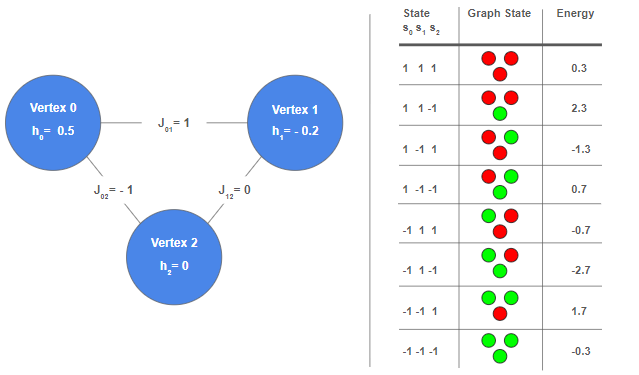
**Left:** a visualization of the N=3 Ising model instance as a 3-vertex complete graph, with h and J terms as labels on vertices and edges respectively. **Right:** an enumeration of all 2³=8 possible states and their energies, calculated by using the Ising model equation. For the graph state, I colored the vertices red for s=+1 and green for s=-1, because I thought it looked cheery! You can see that for this instance, the lowest energy state is s₀=-1, s₁=+1, and s₂=-1 with an energy of -2.7.

From Energies to Probabilities

The Ising model gives us a way to calculate the energies of all the 2ᴺ possible states of an system of N two-state objects. But what’s that good for?

One of the things we might want to know is what the probabilities of seeing each of the possible states are, if we measured them. In the general case, we could define a probability distribution, which is a function that returns a probability for each possible state of the system. The probabilities for all of the possible states have to add up to 1 (that’s how probability works!).

This general case has a very important special case, which is called the Boltzmann distribution. This is a probability distribution, but with the added feature that all states with the same energy are equally likely, and states with lower energies are exponentially more probable than states with higher energies. This is the mathematical formula for the Boltzmann distribution for an N-object system, which converts energies (on the right hand side) to probabilities (the left hand side).

Here k is a constant, T is a positive real number parameter (temperature), and Z is a normalizing factor called the partition function that ensures that the sum over all the probabilities is 1. In the general case computing Z is intractable, but this won’t matter for us as what we really care about is that the probabilities are proportional to the exponential term.

The Boltzmann distribution is the probability distribution that maximizes the entropy of our system. There’s a very important principle in physics called the second law of thermodynamics, which says that time is the thing that drives systems into higher and higher entropy states, and ultimately into thermal equilibrium (the maximum entropy state expressed in the Boltzmann distribution). The second law says that if we wait long enough, and our N objects are a closed system (they don’t interact with anything else), eventually they will have Boltzmann statistics. I don’t want to go too far down into the weeds here, but you can think of the notion of temperature itself being defined by the properties of maximum entropy systems that have the statistics of the Boltzmann distribution.

Back to Our Coin Flip Game

In my last post we talked about what correlations are by thinking about a game where you and I both flip quarters, and I win if they land heads/heads or tails/tails and you win if they land heads/tails or tails/heads. Let’s take a look at that game through the lens of the Ising Model and the Boltzmann distribution.

First, the abstract objects in the Ising Model are now the quarters, and their two states are just heads = +1 and tails = -1. We are assuming each quarter is unbiased (each is equally likely to give heads or tails). So we will set all the h values to zero. But we were playing with the relative coupling by using that ungodly stick contraption! So let’s keep the coupling term. This then gives an Ising Model with energy E(s₀, s₁) = J₀₁*s₀*s₁, and the Boltzmann probabilities

First, let’s say the coupling between the two quarters is zero (J₀₁=0). Looking at the above formula, the exponential of zero is just 1, so each of the probabilities has to be equal for each of the states, and p(heads, heads) = p(heads, tails) = p(tails, heads) = p(tails, tails) = 1/4. (It has to be 1/4 because there are four states and they all have to add up to 1). It doesn’t matter what the temperature parameter is — zero coupling means the objects don’t interact, and since each individually is heads half the time, this makes sense as an answer!

Next, let’s set the coupling strength to be positive (J₀₁/kT=+1). In this case staring at the probabilities we get exp(-1) for s₀ and s₁ the same sign, and exp(+1) for s₀ and s₁ different. Because exp(+1) > exp(-1) this means that for J₀₁/kT positive, states with s₀ and s₁ different (ie one coin lands heads up and one coin lands tails up) are more likely. How much more? This depends on the value of the number J₀₁/kT. As it goes to infinity (for example, as we lower temperature for a fixed value of J₀₁), the difference in probability increases exponentially, and becomes overwhelmingly probable that we will only see heads/tails or tails/heads. So as users of this model, we have a way to tune ‘how much’ one type of result is favored over another, by tuning the values of J₀₁ and/or T. In the previous blog post, sticking the coins to the stick was kind of like taking the ratio J₀₁/kT to infinity.

Similarly if we set the coupling strength to be negative (J₀₁/kT=-1), the same story applies except now it’s the states where the coins read the same that are lower energy.

What Happens With The N=3 Example We Just Looked At?

Let’s use a ‘kind of low but not too low’ temperature, where |J₀₁|/kT=2. Plugging this value into the Boltzmann distribution allows us to go from energies to probabilities for the example we just did; here’s the results!

You can see that the lower the energy, the higher the probability of that state. The probability of being in the lowest energy state here is about 91.7% for the temperature we chose. If we lowered the temperature, this would go up. If we raised the temperature, it would go down. Eventually if the temperature is high enough, all the states become equally likely, and the energy differences don’t matter!

What ‘Sampling From a Probability Distribution’ Means

Why do we measure things at all? Ultimately the answer is ‘we don’t know what we will see’. If we knew what we’d measure, what would the point be of measuring it? For example in the case of flipping a coin, we do the coin flip exactly because we don’t know whether it will land heads or tails. If we think of a simple model of the coin, like the one we built here (the Ising model and a Boltzmann distribution), an actual real-world coin toss is an example of sampling from a probability distribution. This is a very important idea. In a model of the world where the best we can do is provide probabilities for things (like the Boltzmann distribution gives us!), we don’t actually know which result we will see, because the model grounds out in probabilities.

There’s nothing ‘under’ something like the Boltzmann distribution that tells us what exactly we will see when we measure the state of the objects, just probabilities. When we actually look at the objects to see which state they are in, we are drawing a sample from this distribution. In practice, when we use the model itself, this means generating a bunch of random numbers in a computer, and using those random numbers to get a sample.

In the N=3 example I gave, if we want to ‘draw a sample’ from this distribution, we generate a random number in the range 0 to 1, and then based on that random number we return one of the possible states. We might get even the lowest probability state! If we draw a lot of samples, we should start seeing the underlying probability distribution emerge. For fair coin tosses, this means that as we toss the coin more and more, the probability of getting heads should go to 50%, which is an empirical measurement of the probability of getting that state.

So when you read or hear about ‘sampling from a probability distribution’, think back to a sample being an actual instance of a coin toss, or an actual measurement of the states of our N objects. Every time you draw a sample, you’ll in general get a different answer, with each sample’s probability given by whatever its probability distribution is.

A Weird Perspective To Think About

When we measure the state of a system where the outcome is probabilistic, we can think of the different possible outcomes as actions the Universe can choose from. We could think of the Universe having agency, and choice.

For example, we could think of the 8 possible states of the N=3 system above as 8 different actions the Universe could decide to take, where it decides which of them to take when we measure the system’s state.

This is admittedly a weird thing to think about. The only reason I‘m bringing it up is that choosing which action to take for a software agent is also a process that ‘bottoms out’ in probabilities.